Text Analysis and Distant Reading using R

Introduction

This tutorial introduces Text Analysis (see Bernard and Ryan 1998; Kabanoff 1997; Popping 2000), i.e. computer-based analysis of language data or the (semi-)automated extraction of information from text. While Text Analysis encompasses a wide range of methods, this tutorial will only serve as a very basic introduction that highlights selected, commonly used techniques. The entire code for the sections below can be downloaded here.

Since Text Analysis extracts and analyses information from language data, it can be considered a derivative of computational linguistics or an application of Natural Language Processing (NLP) to HASS research. As such, Text Analysis represents the application of computational methods in the humanities. The advantage of Text Analysis over manual or traditional techniques (close reading) lies in the fact that Text Analysis allows the extraction of information from large sets of textual data and in a replicable manner. Other terms that are more or less synonymous with Text Analysis are Text Mining, Text Analytics, and Distant Reading. In some cases, Text Analysis is considered more qualitative while Text Analytics is considered to be quantitative. This distinction is not taken up here as Text Analysis, while allowing for qualitative analysis, builds upon quantitative information, i.e. information about frequencies or conditional probabilities.

Distant Reading is a cover term for applications of Text Analysis that allow to investigate literary and cultural trends using text data. Distant Reading contrasts with close reading, i.e. reading texts in the traditional sense whereas Distant Reading refers to the analysis of large amounts of text. Text Analysis and distant reading are similar with respect to the methods that are used but different with respect to their outlook. The outlook of distant reading is to extract information from text without close reading, i.e. reading the document(s) itself but rather focusing on emerging patterns in the language that is used.

Text Analysis or Distant Reading are rapidly growing in use and gaining popularity in the humanities because textual data is readily available and because computational methods can be applied to a huge variety of research questions. The attractiveness of computational text analysis is thus based on the availability of (large amounts of) digitally available texts and in their capability to provide insights that cannot be derived from close reading techniques.

While rapidly growing as a valid approach to analyzing textual data, Text Analysis is critizised for lack of "quantitative rigor and because its findings are either banal or, if interesting, not statistically robust (see here. This criticism is correct in that most of the analysis that performed in Computational Literary Studies (CLS) are not yet as rigorous as analyses in fields that have a longer history of computational based, quantitative research, such as, for instance, corpus linguistics. However, the practices and methods used in CLS will be refined, adapted and show a rapid increase in quality if more research is devoted to these approaches. Also, Text Analysis simply offers an alternative way to analyze texts that is not in competition to traditional techniques but rather complements them.

Given it relatively recent emergence, so far, most of the applications of Text Analysis are based upon a relatively limited number of key procedures or concepts (e.g. concordancing, word frequencies, annotation or tagging, parsing, collocation, text classification, Sentiment Analysis, Entity Extraction, Topic Modeling, etc.). In the following, we will explore these procedures and introduce some basic tools that help you perform the introduced tasks.

Text Analysis at UQ

The UQ Library offers a very handy and attractive summary of resources, concepts, and tools that can be used by researchers interested in Text Analysis and Distant Reading. Also, the UQ library site offers short video introductions and addresses issues that are not discussed here such as copyright issues, data sources available at the UQ library, as well as social media and web scaping.

In contrast to the UQ library site, the focus of this introduction lies on the practical how-to of text analysis. this means that the following concentrates on how to perform analyses rather than discussing their underlying concepts or evaluating their scientific merits.

Tools versus Scripts

It is perfectly fine to use tools for the analyses exemplified below. However, the aim here is not primarily to show how to perform text analyses but how to perform text analyses in a way that complies with practices that guarantee sustainable, transparent, reproducible research. As R code can be readily shared and optimally contains all the data extraction, processing, visualization, and analysis steps, using scripts is preferable over using (commercial) software.

In addition to being not as transparent and hindering reproduction of research, using tools can also lead to dependencies on third parties which does not arise when using open source software.

Finally, the widespread use of R particularly among data scientists, engineers, and analysts reduces the risk of software errors as a very active community corrects flawed functions typically quite rapidly.

Preparation and session set up

This tutorial is based on R. If you have not installed R or are new to it, you will find an introduction to and more information how to use R here. For this tutorials, we need to install certain packages from an R library so that the scripts shown below are executed without errors. Before turning to the code below, please install the packages by running the code below this paragraph. If you have already installed the packages mentioned below, then you can skip ahead and ignore this section. To install the necessary packages, simply run the following code - it may take some time (between 1 and 5 minutes to install all of the packages so you do not need to worry if it takes some time).

# install packages
install.packages("DT")
install.packages("knitr")
install.packages("kableExtra")
install.packages("quanteda")
install.packages("tidyverse")
install.packages("tm")
install.packages("tidytext")
install.packages("wordcloud2")
install.packages("scales")
install.packages("quanteda.textstats")
install.packages("quanteda.textplots")
install.packages("tidyr")
install.packages("cluster")
install.packages("class")
install.packages("NLP")
install.packages("openNLP")
install.packages("openNLPdata")
install.packages("pacman")
# install klippy for copy-to-clipboard button in code chunks
remotes::install_github("rlesur/klippy")

Now that we have installed the packages, we can activate them as shown below.

# set options
options(stringsAsFactors = F)
options(scipen = 999)
options(max.print=1000)
# load packages
library(tidyverse)
library(flextable)
library(quanteda)
library(tm)
library(tidytext)
library(wordcloud2)
library(scales)
library(quanteda.textstats)
library(quanteda.textplots)
library(tidyr)
library(cluster)
library(class)
library(NLP)
library(openNLP)
library(openNLPdata)
library(pacman)
pacman::p_load_gh("trinker/entity")
# activate klippy for copy-to-clipboard button
klippy::klippy()

Once you have installed R and RStudio and once you have also initiated the session by executing the code shown above, you are good to go.

1 Concordancing

In Text Analysis, concordancing refers to the extraction of words from a given text or texts (Lindquist 2009). Commonly, concordances are displayed in the form of key-word in contexts (KWIC) where the search term is shown with some preceding and following context. Thus, such displays are referred to as key word in context concordances. A more elaborate tutorial on how to perform concordancing with R is available here.

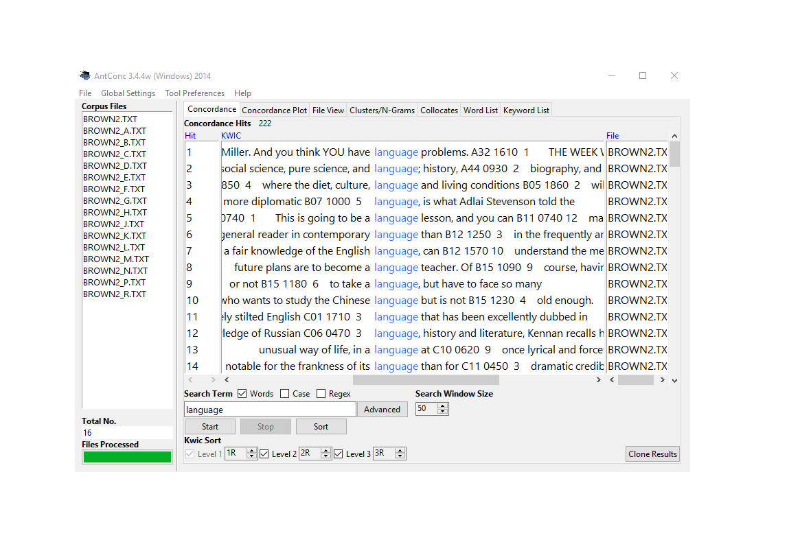
Concordancing is helpful for seeing how the term is used in the data, for inspecting how often a given word occurs in a text or a collection of texts, for extracting examples, and it also represents a basic procedure and often the first step in more sophisticated analyses of language data.

In the following, we will use R to create KWICs displays of the term organism and the phrase natural selection using Charles Darwin’s On the origin of species by means of natural selection.

We begin by loading the quanteda package that we will use for generating the KWICs and the tidyverse package that we use to process the data. In addition, we load the data which represents the text of Charles Darwin’s On the Origin of Species. For the present tutorial, we load data that is available on the LADAL GitHUb repository. If you want to know how to load your own data, have a look at this tutorial.

# load text
darwin <- readLines("https://slcladal.github.io/data/origindarwin.txt")

The data still consists of short text snippets which is why we collapse these snippets and then split the collapsed data into chapters.

# combine and split into chapters
darwin_chapters <- darwin %>%
  # paste all texts together into one long text
  paste0(collapse = " ") %>%
  # replace Chapter I to Chapter XVI with qwertz 
  stringr::str_replace_all("(CHAPTER [XVI]{1,7}\\.{0,1}) ", "qwertz\\1") %>%
  # convert text to lower case
  tolower() %>%  
  # split the long text into chapters
  stringr::str_split("qwertz") %>%
  # unlist the result (convert into simple vector)
  unlist()

Once we have split the data into chapters, we perform the concordancing and extract the KWICs. To create these kwics, we use the kwic function from the quanteda package. This function takes the data (x), the search pattern (pattern), and the window size as its main arguments.

To start with, we generate kwics for the term organism as shown below.

# create kwic
kwic_o <- quanteda::kwic(x = darwin_chapters, # define text(s) 
                         # define pattern
                          pattern = "organism",
                         # define window size
                          window = 5) %>%
  # convert into a data frame
  as.data.frame() %>%
  # remove superfluous columns
  dplyr::select(-to, -from, -pattern)

We can also use regular expressions in our search to extract not only organism but also organisms and organic. When using a regular expression in the pattern argument, we need to specify the valuetype as regex (as shown below).

# create kwic
kwic_os <- quanteda::kwic(x = darwin_chapters, 
                          pattern = "organi.*",
                          window = 5,
                          valuetype = "regex") %>%
  # convert into a data frame
  as.data.frame() %>%
  # remove superfluous columns
  dplyr::select(-to, -from, -pattern)

When search for expressions that represent phrase and that consists out of several elements such as natural selection, we also need to specify that we are looking for a phrase in the pattern argument.

# create kwic
kwic_ns <- quanteda::kwic(x = darwin_chapters, 
                          pattern = quanteda::phrase("natural selection"),
                          window = 5) %>%
  # convert into a data frame
  as.data.frame() %>%
  # remove superfluous columns
  dplyr::select(-to, -from, -pattern)

We could now continue and analyze how Darwin used the phrase natural selection or we could go about investigating how Darwin has used the term organism.

2 Word Frequency

Almost all methods used in text analytics rely on frequency information. Thus, fending out out frequent words are in a text is a fundamental technique in text analytics. In fact, frequency information lies at the very core of Text Analysis. Such frequency information often comes in the form of word frequency lists, i.e. lists of word forms and their frequency in a given text or collection of texts.

As extracting word frequency lists is very important, we will now We will now extract a frequency list from a corpus.

In a first step, we load a corpus, convert everything to lower case, remove non-word symbols (including punctuation), and split the corpus data into individual words.

# load and process corpus
darwin_words <- darwin  %>%
  # convert everything to lower case
  tolower() %>%
  # remove non-word characters
  str_replace_all("[^[:alpha:][:space:]]*", "")  %>%
  tm::removePunctuation() %>%
  stringr::str_squish() %>%
  stringr::str_split(" ") %>%
  unlist()

Now that we have a vector of words, we can easily create a table representing a word frequency list (as shown below).

# create table
wfreq <- darwin_words %>%
  table() %>%
  as.data.frame() %>%
  arrange(desc(Freq)) %>%
  dplyr::rename(word = 1,
                frequency = 2)

The most frequent words are all function words which are often not meaningful or useful for an analysis. Thus, we now remove these function words (also called stopwords) from the frequency list and inspect the list without stopwords.

# create table wo stopwords
wfreq_wostop <- wfreq %>%
  anti_join(stop_words, by = "word") %>%
  dplyr::filter(word != "")

Such word frequency lists can be visualized in various ways. The most common way to visualize word frequency lists is in the form of bargraphs.

wfreq_wostop %>%
  head(10) %>%
  ggplot(aes(x = reorder(word, -frequency, mean), y = frequency)) +
  geom_bar(stat = "identity") +
  labs(title = "10 most frequent non-stop words in \nCharles Darwin's *Origin of Species*",
       x = "") +
  theme(axis.text.x = element_text(angle = 45, size = 12, hjust = 1))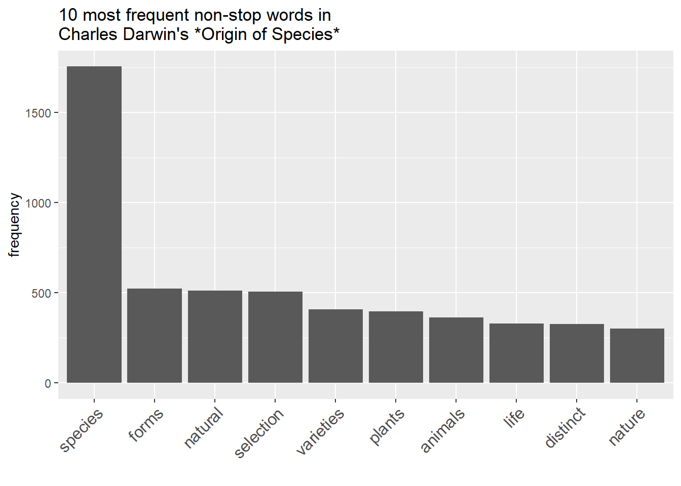

Wordclouds

Alternatively, word frequency lists can be visualized, although less informative, as word clouds.

# create wordcloud
wordcloud2(wfreq_wostop[1:100,],
           shape = "diamond",
           color = scales::viridis_pal()(8)
          )

Another variant of word clouds, so-called comparison clouds, Word lists can be used to determine differences between texts. For instance, we can load different texts and check whether they differ with respect to word frequencies. To show this, we load Herman Melville’s Moby Dick, George Orwell’s 1984, and we also use Darwin’s Origin.

In a first step, we load these texts and collapse them into single documents.

# load data
orwell <- readLines("https://slcladal.github.io/data/orwell.txt") %>%
  paste0(collapse = " ")
melville <- readLines("https://slcladal.github.io/data/melvillemobydick.txt") %>%
  paste0(collapse = " ")
darwin_doc <- paste0(darwin, collapse = " ")

Now, we generate a corpus object from these texts and create a variable with the author name.

corp_dom <- quanteda::corpus(c(darwin_doc, orwell, melville)) 
attr(corp_dom, "docvars")$Author = c("Darwin", "Orwell", "Melville")

Now, we can remove so-called stopwords (non-lexical function words) and punctuation and generate the comparison cloud.

corp_dom  %>%
    quanteda::tokens(remove_punct = TRUE) %>%
    quanteda::tokens_remove(stopwords("english")) %>%
    quanteda::dfm() %>%
    quanteda::dfm_group(groups = corp_dom$Author) %>%
    quanteda::dfm_trim(min_termfreq = 200, verbose = FALSE) %>%
    quanteda.textplots::textplot_wordcloud(comparison = TRUE, 
                                 max_words = 100,
                                 max_size = 6)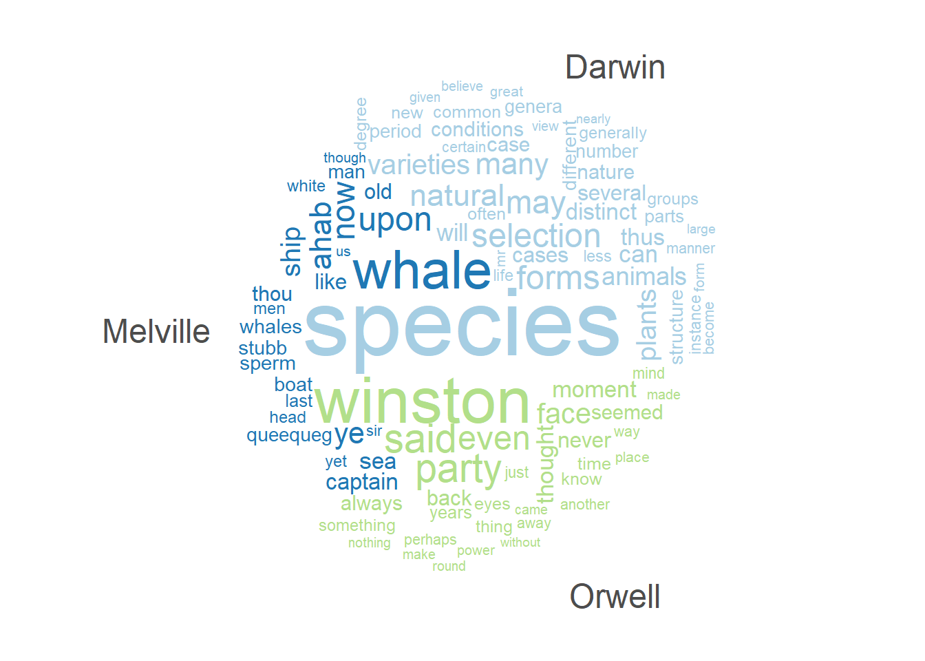

Frequency changes

We can also investigate the use of the term organism across chapters in Darwin’s Origin. In a first step, we extract the number of words in each chapter.

# extract number of words per chapter
Words <- darwin_chapters %>%
  stringr::str_split(" ")  %>%
  lengths()
# inspect data
Words

##  [1]  1856 14065  7456  7136 22317 13916 17781 19055 15847 14741 13313 12996
## [13] 13753  9817 20967 12987

Next, we extract the number of matches in each chapter.

# extract number of matches per chapter
Matches <- darwin_chapters %>%
  stringr::str_count("organism[s]{0,1}")
# inspect the number of matches per chapter
Matches

##  [1]  0  5  3  3  9  3  3  3  0  1  6  6 10  5  8  7

Now, we extract the names of the chapters and create a table with the chapter names and the relative frequency of matches per 1,000 words.

# extract chapters
Chapters <- darwin_chapters %>%
  stringr::str_replace_all("(chapter [xvi]{1,7})\\.{0,1} .*", "\\1")
Chapters <- dplyr::case_when(nchar(Chapters) > 50 ~ "chapter 0", TRUE ~ Chapters)
Chapters

##  [1] "chapter 0"    "chapter i"    "chapter ii"   "chapter iii"  "chapter iv"  
##  [6] "chapter v"    "chapter vi"   "chapter vii"  "chapter viii" "chapter ix"  
## [11] "chapter x"    "chapter xi"   "chapter xii"  "chapter xiii" "chapter xiv" 
## [16] "chapter xv"

# create table of results
tb <- data.frame(Chapters, Matches, Words) %>%
  dplyr::mutate(Frequency = round(Matches/Words*1000, 2))

We can now visualize the relative frequencies of our search word per chapter.

# create plot
ggplot(tb, aes(x = Chapters, y = Frequency, group = 1)) + 
  geom_smooth(color = "purple") +
  geom_line(color = "darkgray") +         
  guides(color=guide_legend(override.aes=list(fill=NA))) +
  theme_bw() +
  theme(axis.text.x = element_text(angle = 45, hjust = 1))+
  scale_y_continuous(name ="Relative Frequency (per 1,000 words)")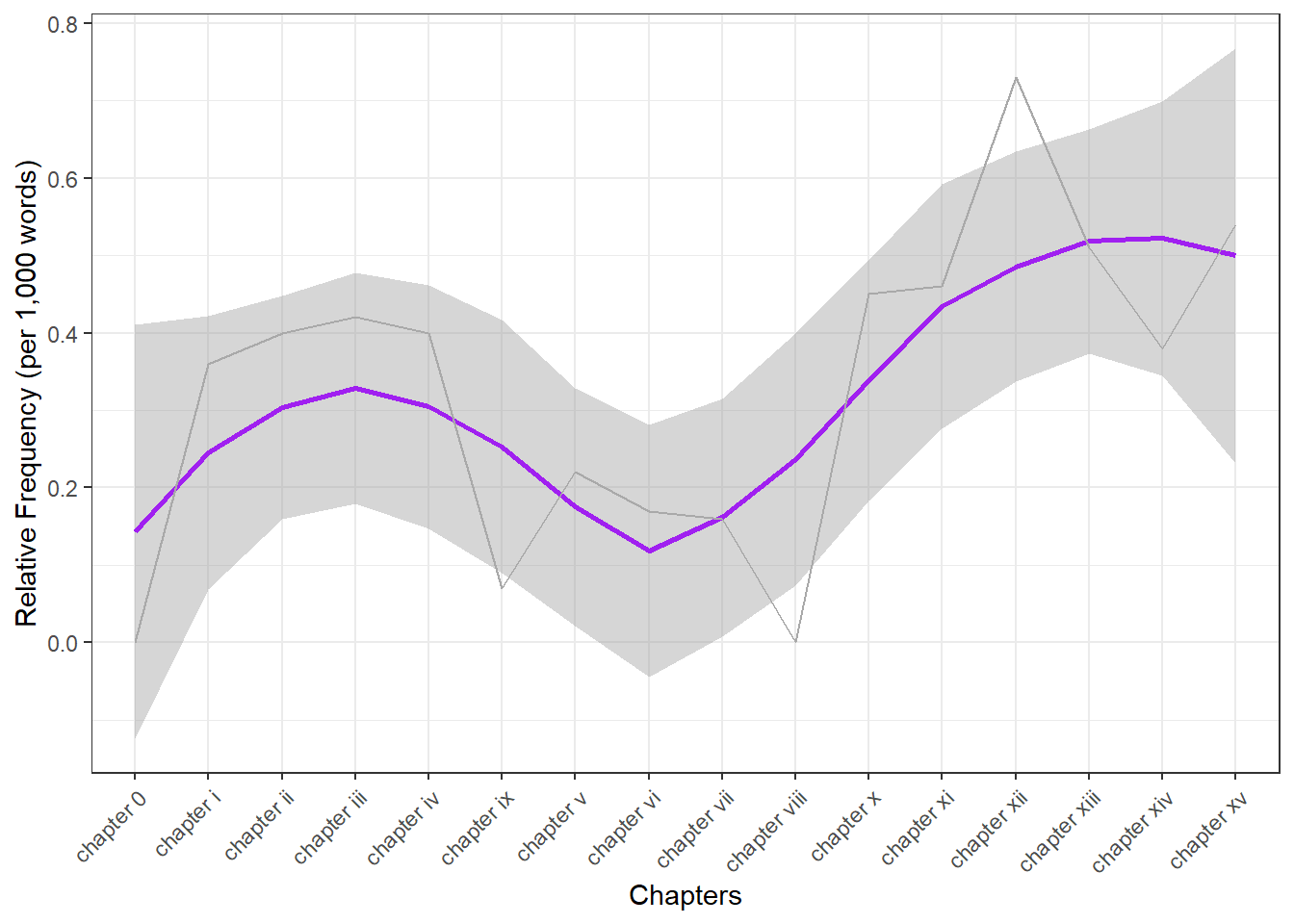

Dispersion plots

To show when in a text or in a collection of texts certain terms occur, we can use dispersion plots. The quanteda package offers a very easy-to-use function textplot_xray to generate dispersion plots.

# add chapter names
names(darwin_chapters) <- Chapters
# generate corpus from chapters
darwin_corpus <- quanteda::corpus(darwin_chapters)
# generate dispersion plots
quanteda.textplots::textplot_xray(kwic(darwin_corpus, pattern = "organism"),
              kwic(darwin_corpus, pattern = "selection"),
              sort = T)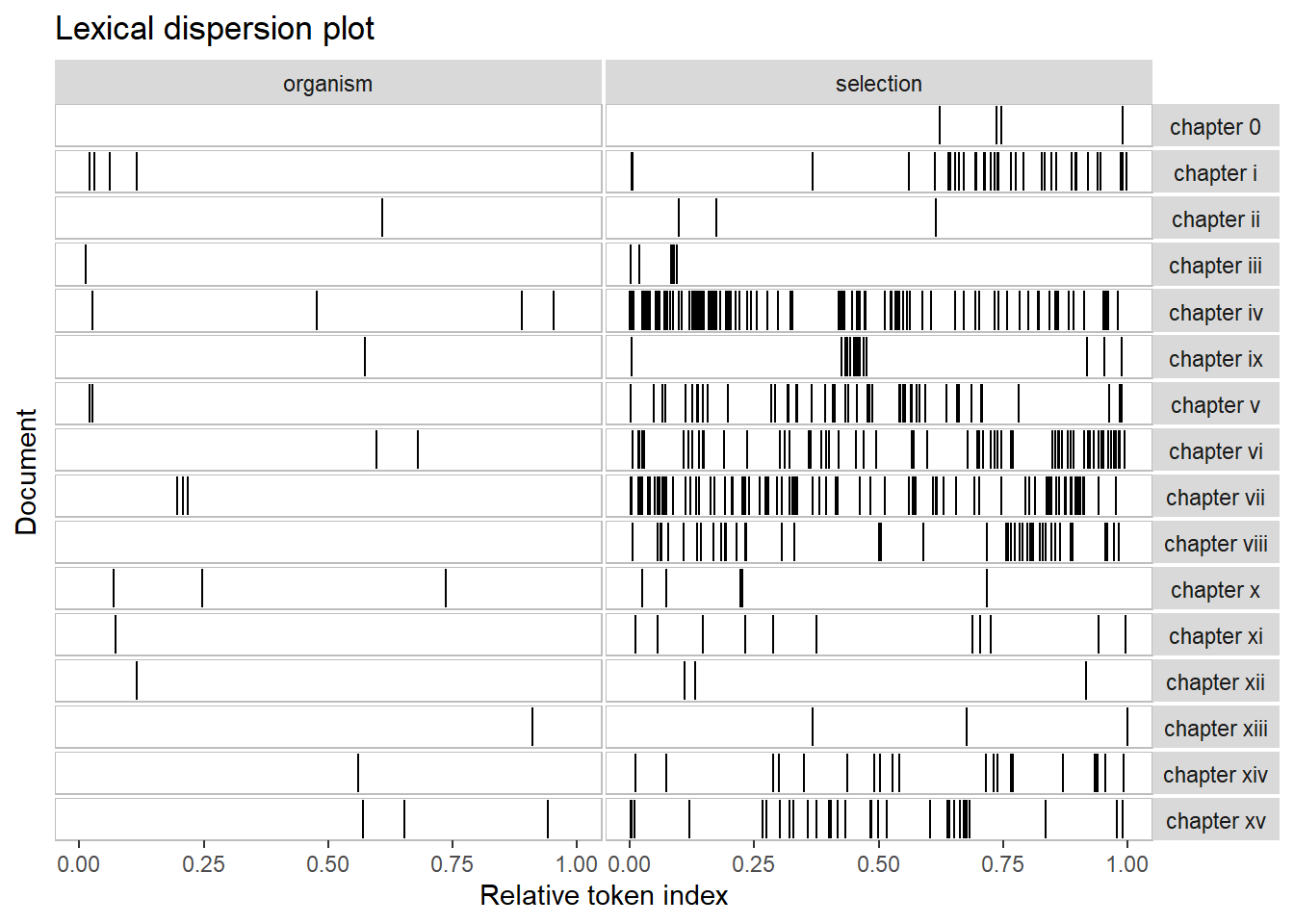

Over- and underuse

Frequency information can also tell us something about the nature of a text. For instance, private dialogues will typically contain higher rates of second person pronouns compared with more format text types, such as, for instance, scripted monologues like speeches. For this reason, word frequency lists can be used in text classification and to determine the formality of texts.

As an example, below you find the number of the second person pronouns you and your and the number of all words except for these second person pronouns in private dialogues compared with scripted monologues in the Irish component of the International Corpus of English (ICE). In addition, the tables shows the percentage of second person pronouns in both text types to enable seeing whether private dialogues contain more of these second person pronouns than scripted monologues (i.e. speeches).

This simple example shows that second person pronouns make up 2.6 percent of all words that are used in private dialogues while they only amount to 0.63 percent in scripted speeches. A handy way to present such differences visually are association and mosaic plots.

d <- matrix(c(6761, 659, 259625, 105295), nrow = 2, byrow = T)
colnames(d) <- c("D", "M")
rownames(d) <- c("you, your", "Other words")
assocplot(d)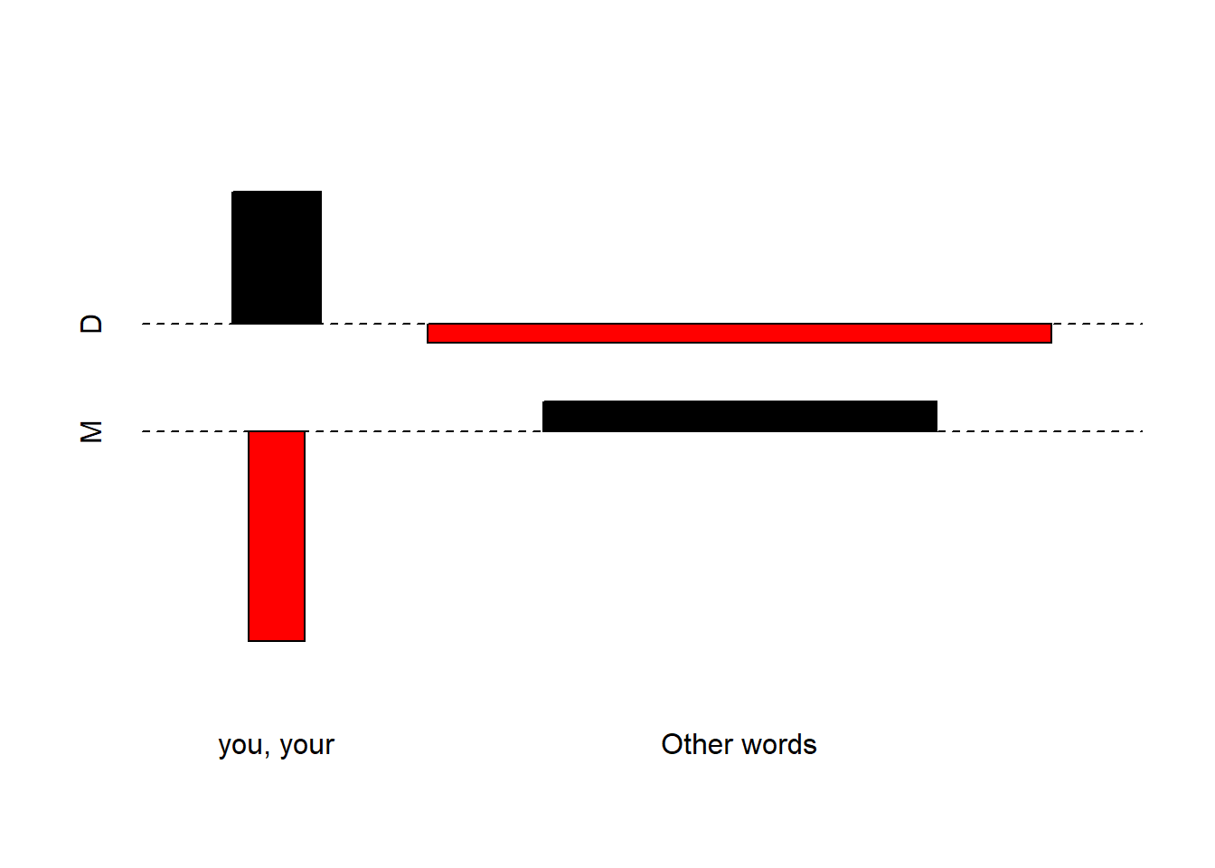

Bars above the dashed line indicate relative overuse while bars below the line suggest relative under-use. Therefore, the association plot indicates under-use of you and your and overuse of other words in monologues while the opposite trends holds true for dialogues, i.e. overuse of you and your and under-use of Other words.

3 N-grams, Collocations, and Keyness

Collocation refers to the co-occurrence of words. A typical example of a collocation is Merry Christmas because the words merry and Christmas occur together more frequently together than would be expected by chance, if words were just randomly stringed together.

N-grams are related to collocates in that they represent words that occur together (bi-grams are two words that occur together, tri-grams three words and so on). Fortunately, creating N-gram lists is very easy. We will use the Origin to create a bi-gram list. We can simply take each word and combine it with the following word.

# create data frame
darwin_bigrams <- data.frame(darwin_words[1:length(darwin_words)-1], 
                       darwin_words[2:length(darwin_words)]) %>%
  dplyr::rename(Word1 = 1,
                Word2 = 2) %>%
  dplyr::mutate(Bigram = paste0(Word1, " ", Word2)) %>%
  dplyr::group_by(Bigram) %>%
  dplyr::summarise(Frequency = n()) %>%
  dplyr::arrange(-Frequency)

Both N-grams and collocations are not only an important concept in language teaching but they are also fundamental in Text Analysis and many other research areas working with language data. Unfortunately, words that collocate do not have to be immediately adjacent but can also encompass several slots which makes it harder to retrieve of collocates that are not adjacent- We will find out how to identify non-adjacent collocates in the next section.

Finding collocations

There are various techniques for identifying collocations. To identify collocations without having a pre-defined target term, we can use the textstat_collocations function from the quanteda.textstats package.

However, before we can apply that function and start identifying collocations, we need to process the data to which we want to apply this function. In the present case, we will apply that function to the sentences in Charles Darwin’s Origin which we extract in the code chunk below.

darwin_sentences <- darwin %>%
  tolower() %>%
  paste0(collapse= " ") %>%
  stringr::str_split(fixed(".")) %>%
  unlist() %>%
  tm::removePunctuation() %>%
  stringr::str_squish()

From the output shown above, we also see that splitting texts simply by full stops is not optimal as it produces some unwarranted artifacts like the “sentences” that consist of single characters (due to the name of the H.M.S. Beagle - the ship on which Darwin traveled when he explored the southern hemisphere). Fortunately, these errors do not really matter in the case of our example.

Now that we have split Darwin’s Origin into sentences, we can tokenize these sentences and apply the textstat_collocations function which identifies collocations.

# create a token object
darwin_tokens <- tokens(darwin_sentences, remove_punct = TRUE) %>%
  tokens_remove(stopwords("english"))
# extract collocations
darwin_coll <- textstat_collocations(darwin_tokens, size = 2, min_count = 20)

The resulting table shows collocations in Darwin’s Origin descending by collocation strength.

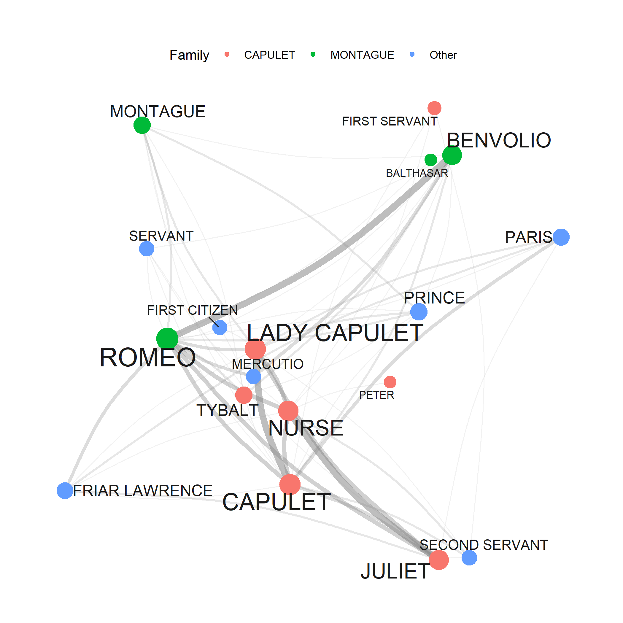
Visualizing Collocation Networks

Network graphs are a very useful and flexible tool for visualizing relationships between elements such as words, personas, or authors. This section shows how to generate a network graph for collocations of the term organism using the quanteda package.

In a first step, we generate a document-feature matrix based on the sentence sin Charles Darwin’s Origin. A document-feature matrix shows how often elements (here these elements are the words that occur in the Origin) occur in a selection of documents (here these documents are the sentences in the Origin).

# create document-feature matrix
darwin_dfm <- darwin_sentences %>% 
    quanteda::dfm(remove = stopwords('english'), remove_punct = TRUE) %>%
    quanteda::dfm_trim(min_termfreq = 10, verbose = FALSE)

As we want to generate a network graph of words that collocate with the term organism, we use the calculateCoocStatistics function to determine which words most strongly collocate with our target term (organism).

# load function for co-occurrence calculation
source("https://slcladal.github.io/rscripts/calculateCoocStatistics.R")
# define term
coocTerm <- "organism"
# calculate co-occurrence statistics
coocs <- calculateCoocStatistics(coocTerm, darwin_dfm, measure="LOGLIK")
# inspect results
coocs[1:20]

##  conditions      nature    relation   relations    physical      action 
##   56.666499   34.485146   25.478537   22.836815   21.740633   20.608922 
##        life     bearing   important        many      direct   colonists 
##   18.807464   16.246065   15.812686   13.488588   12.705077   11.300306 
## competition      nearly     welfare     require     altered   different 
##   11.140540   10.945131   10.886868   10.514045   10.174698    9.774481 
## improvement     rapidly 
##    9.576033    9.576033

We now reduce the document-feature matrix to contain only the top 20 collocates of organism (plus our target word organism).

redux_dfm <- dfm_select(darwin_dfm, 
                        pattern = c(names(coocs)[1:20], "organism"))

Now, we can transform the document-feature matrix into a feature-co-occurrence matrix as shown below. A feature-co-occurrence matrix shows how often each element in that matrix co-occurs with every other element in that matrix.

tag_fcm <- fcm(redux_dfm)

Using the feature-co-occurrence matrix, we can generate the network graph which shows the terms that collocate with the target term organism with the edges representing the co-occurrence frequency. To generate this network graph, we use the textplot_network function from the quanteda.textplots package.

# generate network graph
textplot_network(tag_fcm, 
                 min_freq = 1, 
                 edge_alpha = 0.1, 
                 edge_size = 5,
                 edge_color = "purple",
                 vertex_labelsize = log(rowSums(tag_fcm))*2)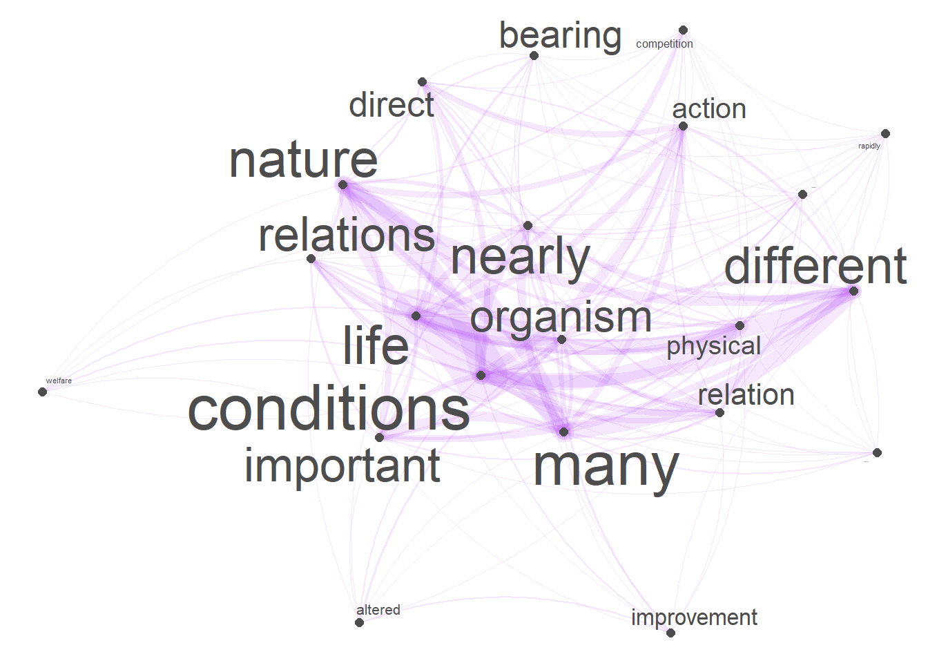

Keyness

Another common method that can be used for automated text summarization is keyword extraction. Keyword extraction builds on identifying words that are particularly associated with a certain text. In other words, keyness analysis aims to identify words that are particularly indicative of the content of a certain text.

Below, we identify key words for Charles Darwin’s Origin, Herman Melville’s Moby Dick, and George Orwell’s 1984. We start by creating a weighted document feature matrix from the corpus containing the three texts.

dfm_authors <- corp_dom %>%
  quanteda::tokens(remove_punct = TRUE) %>%
  quanteda::tokens_remove(stopwords("english")) %>%
  quanteda::dfm() %>%
  quanteda::dfm_weight(scheme = "prop")

In a next step, we use the textstat_frequency function from the quanteda package to extract the most frequent non-stopwords in the three texts.

# Calculate relative frequency by president
freq_weight <- quanteda.textstats::textstat_frequency(dfm_authors, n = 10,
                                            groups = dfm_authors$Author)

Now, we can simply plot the most common words and most indicative non-stop words in the three texts.

ggplot(freq_weight, aes(nrow(freq_weight):1, frequency)) +
     geom_point() +
     facet_wrap(~ group, scales = "free") +
     coord_flip() +
     scale_x_continuous(breaks = nrow(freq_weight):1,
                        labels = freq_weight$feature) +
     labs(x = NULL, y = "Relative frequency")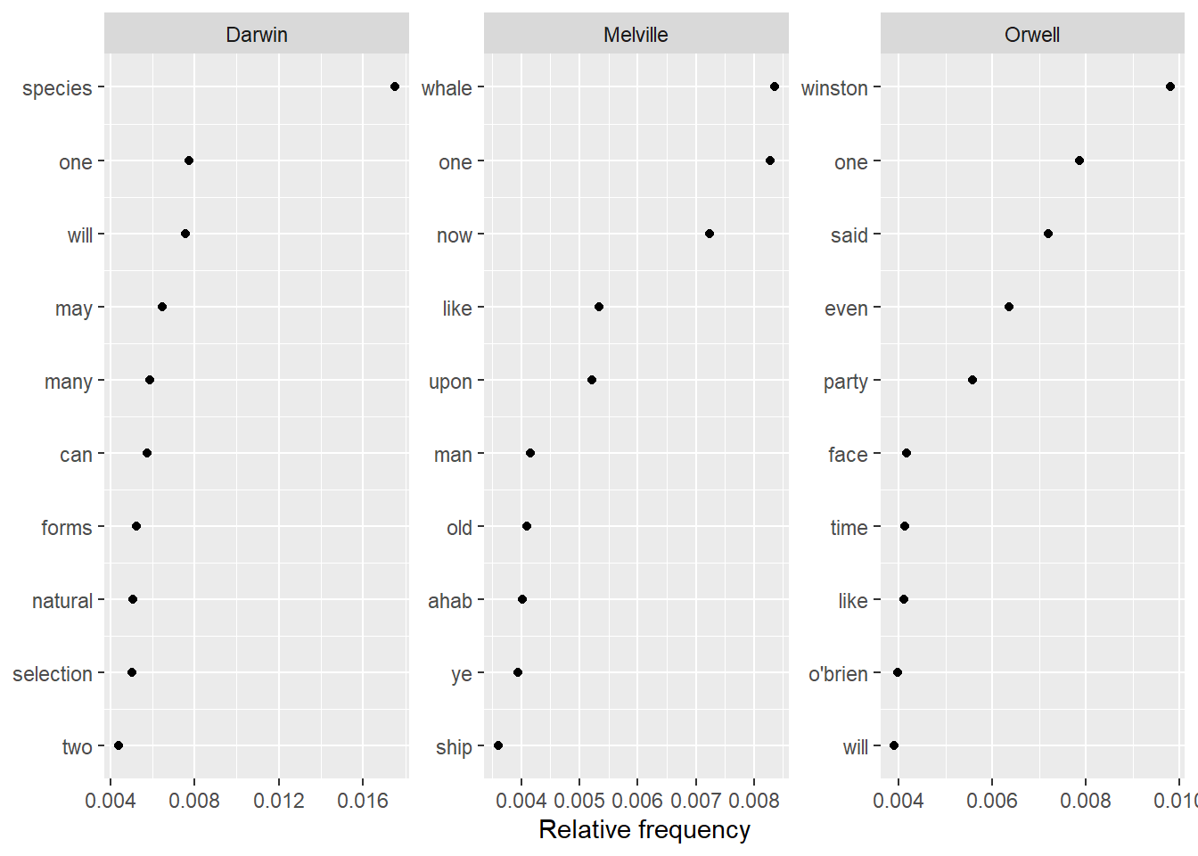

4 Text Classification

Text classification refers to methods that allow to classify a given text to a predefined set of languages, genres, authors, or the like. Such classifications are typically based on the relative frequency of word classes, key words, phonemes, or other linguistic features such as average sentence length, words per line, etc.

As with most other methods that are used in text analysis, text classification typically builds upon a training set that is already annotated with the required tags. Training sets and the features that are derived from these training sets can be created by oneself or one can use build in training sets that are provided in the respective software packages or tools.

In the following, we will use the frequency of phonemes to classify a text. In a first step, we read in a German text, and split it into phonemes.

# read in German text
German <- readLines("https://slcladal.github.io/data/phonemictext1.txt") %>%
  stringr::str_remove_all(" ") %>%
  stringr::str_split("") %>%
  unlist()
# inspect data
head(German, 20)

##  [1] "?" "a" "l" "s" "h" "E" "s" "@" "d" "e" ":" "n" "S" "t" "E" "p" "@" "n" "v"
## [20] "O"

We now do the same for three other texts - an English and a Spanish text as well as one text in a language that we will determine using classification.

# read in texts
English <- readLines("https://slcladal.github.io/data/phonemictext2.txt")
Spanish <- readLines("https://slcladal.github.io/data/phonemictext3.txt")
Unknown <- readLines("https://slcladal.github.io/data/phonemictext4.txt")
# clean, split texts into phonemes, unlist and convert them into vectors
English <- as.vector(unlist(strsplit(gsub(" ", "", English), "")))
Spanish <- as.vector(unlist(strsplit(gsub(" ", "", Spanish), "")))
Unknown <- as.vector(unlist(strsplit(gsub(" ", "", Unknown), "")))
# inspect data
head(English, 20)

##  [1] "D"  "@"  "b"  "U"  "k"  "I"  "z"  "p"  "r"  "\\" "@"  "z"  "E"  "n"  "t" 
## [16] "@"  "d"  "{"  "z"  "@"

We will now create a table that represents the phonemes and their frequencies in each of the 4 texts. In addition, we will add the language and simply the column names.

# create data tables
German <- data.frame(names(table(German)), as.vector(table(German)))
English <- data.frame(names(table(English)), as.vector(table(English)))
Spanish <- data.frame(names(table(Spanish)), as.vector(table(Spanish)))
Unknown <- data.frame(names(table(Unknown)), as.vector(table(Unknown)))
# add column with language
German$Language <- "German"
English$Language <- "English"
Spanish$Language <- "Spanish"
Unknown$Language <- "Unknown"
# simplify column names
colnames(German)[1:2] <- c("Phoneme", "Frequency")
colnames(English)[1:2] <- c("Phoneme", "Frequency")
colnames(Spanish)[1:2] <- c("Phoneme", "Frequency")
colnames(Unknown)[1:2] <- c("Phoneme", "Frequency")
# combine all tables into a single table
classdata <- rbind(German, English, Spanish, Unknown) 

Now, we group the data so that we see, how often each phoneme is used in each language.

# convert into wide format
classdw <- classdata %>%
  spread(Phoneme, Frequency) %>%
  replace(is.na(.), 0)

Now, we need to transform the data again, so that we have the frequency of each phoneme by language as the classifier will use “Language” as the dependent variable and the phoneme frequencies as predictors.

numvar <- colnames(classdw)[2:length(colnames(classdw))]
classdw[numvar] <- lapply(classdw[numvar], as.numeric)
# function for normalizing numeric variables
normalize <- function(x) { (x-min(x))/(max(x)-min(x))   }
# apply normalization
 classdw[numvar] <- as.data.frame(lapply(classdw[numvar], normalize))

Before turning to the actual classification, we will use a cluster analysis to see which texts the unknown text is most similar with.

# remove language column
textm <- classdw[,2:ncol(classdw)]
# add languages as row names
rownames(textm) <- classdw[,1]
# create distance matrix
distmtx <- dist(textm)
# perform clustering
clustertexts <- hclust(distmtx, method="ward.D")  
# visualize cluster result
plot(clustertexts, hang = .25,main = "")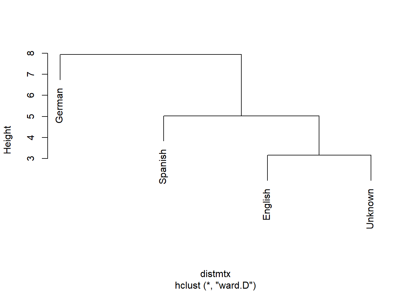           

According to the cluster analysis, the unknown text clusters together with the English texts which suggests that the unknown text is likely to be English.

Before we begin with the actual classification, we will split the data so that we have one data set without “Unknown” (this is our training set) and one data set with only “Unknown” (this is our test set).

# create training set
train <- classdw %>%
  filter(Language != "Unknown")
# create test set
test <- classdw %>%
  filter(Language == "Unknown")

Finally, we can apply our classifier to our data. The classifier we use is a k-nearest neighbor classifier as the underlying function will classify an unknown element given its proximity to the clusters in the training set.

# set seed for reproducibility
set.seed(12345)
# apply k-nearest-neighbor (knn) classifier
prediction <- class::knn(train[,2:ncol(train)], 
                         test[,2:ncol(test)], 
                         cl = train[, 1], 
                         k = 3)
# inspect the result
prediction

## [1] English
## Levels: English German Spanish

Based on the frequencies of phonemes in the unknown text, the knn-classifier predicts that the unknown text is English. This is in fact true as the text is a subsection of the Wikipedia article for Aldous Huxley’s Brave New World. The training texts were German, English, and Spanish translations of a subsection of Wikipedia’s article for Hermann Hesse’s Steppenwolf.

5 Entity Extraction

Named Entity Recognition (NER) (also referred to as named entity extraction or simply as entity extraction) is a text analytic method which allows us to automatically identify or extract named entities from text(s) such as persons, locations, brands, etc.

As such, NER is a process during which textual elements which have characteristics that are common to proper nouns (locations, people, organizations, etc.) rather than other parts of speech, e.g. non-sentence initial capitalization, are extracted from texts. Retrieving entities is common in automated summarization and in Topic Modeling. NER can be achieved by simple feature extraction (e.g. extract all non-sentence initial capitalized words) or with the help of training sets. Using training sets, i.e. texts that are annotated for entities and non-entities, achieves better results when dealing with unknown data and data with inconsistent capitalization.

There are different options to extract entities from texts in R. Here, we will focus on two methods:

1. entity extraction using pacman and entity packages provided by Tyler Rinker which builds on the NLP and openNLP packages; and

2. entity extraction using the NLP and openNLP packages directly.

5.1 NER using pacman

As we have already installed and activated the required packages during the session preparation, we can start right away by loading and cleaning a sample text - which is a summary of Aldous Huxley’s Brave New World.

# load corpus data
text <- readLines("https://slcladal.github.io/data/text4.txt", skipNul = T) %>%
  # clean data
  stringr::str_squish() %>%
  # remove empty elements
  .[. != ""]

We can now extract the entities form that text using the person_entity from the entity package.

# extract person entities
entity::person_entity(text)

## [[1]]
## [1] "Lenina Crowne" "Bernard Marx"  "Bernard"      
## 
## [[2]]
##  [1] "Bernard and" "Linda"       "John"        "John"        "Linda"      
##  [6] "Linda"       "John"        "Shakespeare" "John"        "King Lear"  
## [11] "Juliet"      "John"        "Bernard"     "John"        "John"       
## 
## [[3]]
## [1] "Bernard"     "Linda"       "John"        "Bernard"     "John"       
## [6] "John"        "Shakespeare" "Linda"       "Bernard"    
## 
## [[4]]
## [1] "John"          "Mustapha Mond" "Bernard"       "Bernard"      
## [5] "Bernard"       "John"          "John"          "John"         
## 
## [[5]]
## [1] "John" "John" "John" "John"

We can also extract other types of entities as shown below - I have de-activated the code chunk, but you can run the code and check out the results.

# extract locations
entity::location_entity(text)
entity::organization_entity(text)
entity::date_entity(text)
entity::money_entity(text)
entity::percent_entity(text)

NER using NLP and openNLP

We can also perform NER using the NLP and openNLP packages directly (rather than the pacman and entity packages which are wrapper of the NLP and openNLP packages). This is a bit more complex, but it also allows for more flexibility, e.g. extarcting entities by sentence rather than by text.

# convert text into string
text = as.String(text)
# define annotators
# sentence annotator
sent_annot = openNLP::Maxent_Sent_Token_Annotator()
# word annotator
word_annot = openNLP::Maxent_Word_Token_Annotator()

---

NOTE
I had an issue with the following lines of code because R asked me for a package (openNLPmodels.en) that I could not install for the R version I am currently running (4.1). You can find the language packages for English, Spanish, German, Swedish, Dutch, Italian, Danish, and Polish under: https://slcladal.github.io/packages/ - simply download and install them to the library of your current R version.

The original versions of these packages can be downloaded from https://datacube.wu.ac.at/src/contrib/.

---

Once the openNLPmodels.en model is your R library, you can run the code chunk below.

# location annotator
loc_annot = openNLP::Maxent_Entity_Annotator(kind = "location") 
# person annotator
people_annot = openNLP::Maxent_Entity_Annotator(kind = "person") 
# apply annotations
textanno = NLP::annotate(text, list(sent_annot, word_annot, 
                                        loc_annot, people_annot))

Now that we have annotated the data, we can extract elements that have been identified as locations of persons.

# extract features
k <- sapply(textanno$features, `[[`, "kind")
# extract locations
textlocations = names(table(text[textanno[k == "location"]]))
# extract people
textpeople = names(table(text[textanno[k == "person"]]))
# inspect extract people
textpeople

## [1] "Bernard"       "Bernard Marx"  "John"          "Juliet"       
## [5] "King Lear"     "Linda"         "Mustapha Mond" "Shakespeare"

The output shows that the extraction of people and locations from the example text was successful as we can see various places and persons in the output.

6 Part-of-Speech tagging

A very common procedure to add information to texts is to part-of-speech tag the data, which means to determine to what type of word a specific word belongs. Below, we will add pos-tags to a short English text.

We begin by writing a function which adds part of speech tags to an English text.

# function for pos-tagging
tagPOS <-  function(x, ...) {
  s <- as.String(x)
  word_token_annotator <- Maxent_Word_Token_Annotator()
  a2 <- Annotation(1L, "sentence", 1L, nchar(s))
  a2 <- annotate(s, word_token_annotator, a2)
  a3 <- annotate(s, Maxent_POS_Tag_Annotator(), a2)
  a3w <- a3[a3$type == "word"]
  POStags <- unlist(lapply(a3w$features, `[[`, "POS"))
  POStagged <- paste(sprintf("%s/%s", s[a3w], POStags), collapse = " ")
  list(POStagged = POStagged)
  }

We now apply this function to the text and then display the results.

# load text
text <- readLines("https://slcladal.github.io/data/english.txt")
# pos tagging data
textpos <- tagPOS(text)
# inspect data
textpos

## $POStagged
## [1] "Linguistics/NNP is/VBZ the/DT scientific/JJ study/NN of/IN language/NN and/CC it/PRP involves/VBZ the/DT analysis/NN of/IN language/NN form/NN ,/, language/NN meaning/NN ,/, and/CC language/NN in/IN context/NN ./."

We could, for example, use pos-tagging to check differences in the distribution of word classes across different registers. or to find certain syntactic patterns in a collection of texts.

Citation & Session Info

Schweinberger, Martin. 2021. Text Analysis and Distant Reading using R. Brisbane: The University of Queensland. url: https://slcladal.github.io/textanalysis.html (Version 2021.10.04).

@manual{schweinberger2021ta,
  author = {Schweinberger, Martin},
  title = {Text Analysis and Distant Reading using R},
  note = {https://slcladal.github.io/textanalysis.html},
  year = {2021},
  organization = "The University of Queensland, Australia. School of Languages and Cultures},
  address = {Brisbane},
  edition = {2021.10.04}
}

sessionInfo()

## R version 4.1.1 (2021-08-10)
## Platform: x86_64-w64-mingw32/x64 (64-bit)
## Running under: Windows 10 x64 (build 19043)
## 
## Matrix products: default
## 
## locale:
## [1] LC_COLLATE=German_Germany.1252  LC_CTYPE=German_Germany.1252   
## [3] LC_MONETARY=German_Germany.1252 LC_NUMERIC=C                   
## [5] LC_TIME=German_Germany.1252    
## 
## attached base packages:
## [1] stats     graphics  grDevices utils     datasets  methods   base     
## 
## other attached packages:
##  [1] slam_0.1-48               Matrix_1.3-4             
##  [3] entity_0.1.0              pacman_0.5.1             
##  [5] openNLPdata_1.5.3-4       openNLP_0.2-7            
##  [7] class_7.3-19              cluster_2.1.2            
##  [9] quanteda.textplots_0.94   quanteda.textstats_0.94.1
## [11] scales_1.1.1              wordcloud2_0.2.1         
## [13] tidytext_0.3.1            tm_0.7-8                 
## [15] NLP_0.2-1                 quanteda_3.1.0           
## [17] flextable_0.6.8           forcats_0.5.1            
## [19] stringr_1.4.0             dplyr_1.0.7              
## [21] purrr_0.3.4               readr_2.0.1              
## [23] tidyr_1.1.3               tibble_3.1.4             
## [25] ggplot2_3.3.5             tidyverse_1.3.1          
## 
## loaded via a namespace (and not attached):
##  [1] colorspace_2.0-2     ellipsis_0.3.2       base64enc_0.1-3     
##  [4] fs_1.5.0             rstudioapi_0.13      farver_2.1.0        
##  [7] SnowballC_0.7.0      ggrepel_0.9.1        fansi_0.5.0         
## [10] lubridate_1.7.10     xml2_1.3.2           splines_4.1.1       
## [13] knitr_1.34           jsonlite_1.7.2       rJava_1.0-5         
## [16] broom_0.7.9          dbplyr_2.1.1         compiler_4.1.1      
## [19] httr_1.4.2           backports_1.2.1      assertthat_0.2.1    
## [22] fastmap_1.1.0        cli_3.0.1            htmltools_0.5.2     
## [25] tools_4.1.1          coda_0.19-4          gtable_0.3.0        
## [28] glue_1.4.2           fastmatch_1.1-3      Rcpp_1.0.7          
## [31] cellranger_1.1.0     statnet.common_4.5.0 vctrs_0.3.8         
## [34] nlme_3.1-152         xfun_0.26            stopwords_2.2       
## [37] network_1.17.1       rvest_1.0.1          nsyllable_1.0       
## [40] lifecycle_1.0.1      klippy_0.0.0.9500    hms_1.1.0           
## [43] parallel_4.1.1       RColorBrewer_1.1-2   yaml_2.2.1          
## [46] gdtools_0.2.3        stringi_1.7.4        highr_0.9           
## [49] tokenizers_0.2.1     zip_2.2.0            rlang_0.4.11        
## [52] pkgconfig_2.0.3      systemfonts_1.0.2    evaluate_0.14       
## [55] lattice_0.20-44      htmlwidgets_1.5.4    labeling_0.4.2      
## [58] tidyselect_1.1.1     magrittr_2.0.1       R6_2.5.1            
## [61] generics_0.1.0       sna_2.6              DBI_1.1.1           
## [64] pillar_1.6.3         haven_2.4.3          withr_2.4.2         
## [67] mgcv_1.8-36          proxyC_0.2.1         janeaustenr_0.1.5   
## [70] modelr_0.1.8         crayon_1.4.1         uuid_0.1-4          
## [73] utf8_1.2.2           tzdb_0.1.2           rmarkdown_2.5       
## [76] officer_0.4.0        grid_4.1.1           readxl_1.3.1        
## [79] data.table_1.14.0    reprex_2.0.1.9000    digest_0.6.27       
## [82] RcppParallel_5.1.4   munsell_0.5.0        viridisLite_0.4.0

---

Back to top

Back to HOME

---

References

Bernard, H Russell, and Gery Ryan. 1998. “Text Analysis.” Handbook of Methods in Cultural Anthropology 613.

Kabanoff, Boris. 1997. “Introduction: Computers Can Read as Well as Count: Computer-Aided Text Analysis in Organizational Research.” Journal of Organizational Behavior, 507–11.

Lindquist, Hans. 2009. Corpus Linguistics and the Description of English. Edinburgh: Edinburgh University Press.

Popping, Roel. 2000. Computer-Assisted Text Analysis. Sage.