Converting PDFs to txt files with R

Introduction

This tutorial shows how to extract text from one or more pdf-files and then saving the text(s) in txt-files on your computer. The RNotebook for this tutorial can be downloaded here.

Preparation and session set up

This tutorial is based on R. If you have not installed R or are new to it, you will find an introduction to and more information how to use R here. For this tutorials, we need to install certain packages from an R library so that the scripts shown below are executed without errors. Before turning to the code below, please install the packages by running the code below this paragraph. If you have already installed the packages mentioned below, then you can skip ahead and ignore this section. To install the necessary packages, simply run the following code - it may take some time (between 1 and 5 minutes to install all of the libraries so you do not need to worry if it takes some time).

# set options
options(stringsAsFactors = F)          # no automatic data transformation
options("scipen" = 100, "digits" = 12) # suppress math annotation
# install packages
install.packages("pdftools")
install.packages("tidyverse")
install.packages("here")
# install klippy for copy-to-clipboard button in code chunks
remotes::install_github("rlesur/klippy")

Next we activate the packages.

# activate packages
library(pdftools)
library(tidyverse)
library(here)
# activate klippy for copy-to-clipboard button
klippy::klippy()

Once you have installed RStudio and have also initiated the session by executing the code shown above, you are good to go.

How to use the RNotebook for this tutorial

To follow this tutorial interactively (by using the RNotebook - or Rmd for short), follow the instructions listed below.

Data and folder set up

1. Create a folder somewhere on your computer
2. In that folder create a sub-folder called data
3. In that data folder, create a subfolder called PDFs
4. Download and save the following pdf-files in that PDFs folder: pdf0, pdf1, pdf2, and pdf3.

R and RStudio set up

1. Download the RNotebook and save it in the folder you have just created
2. Open RStudio
3. Click on File in the upper left corner of the R Studio interface
4. Click on New Project...
5. Select Existing Directory
6. Browse to the folder you have just created and click on Open
7. Now click on Files above the lower right panel
8. Click on the file pdf2txt.Rmd
   • The Markdown file of this tutorial should now be open in the upper left panel of RStudio. To execute the code which prepare the session, load the data, create the graphs, and perform the statistics, simply click on the green arrows in the top right corner of the code boxes.
   • To render a PDF of this tutorial, simply click on Knit above the upper left panel in RStudio.

Extract text from one pdf

The pdf we will convert is a pdf of the Wikipedia article about corpus linguistics. The first part of that pdf is shown below.

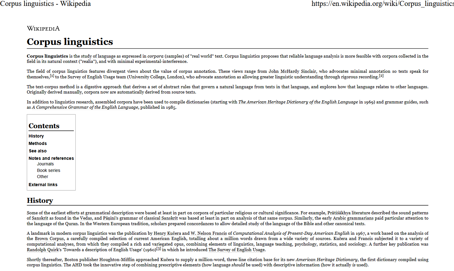
Given that the pdf contains tables, urls, reference, etc., the text that we will extract from the pdf will be rather messy - cleaning the content of the text would be another matter (it would be data processing rather than extraction) and we will thus only focus on the conversion process here and not focus on the data cleaning and processing aspect.

We begin the extraction by defining a path to the pdf. Once we have defined a path, i.e. where R is supposed to look for that file, we continue by extracting the text from the pdf.

# you can use an url or a path that leads to a pdf document
pdf_path <- "https://slcladal.github.io/data/PDFs/pdf0.pdf"
# extract text
txt_output <- pdftools::pdf_text(pdf_path) %>%
  paste0(collapse = " ") %>%
  paste0(collapse = " ") %>%
  stringr::str_squish() 

Extracting text from many pdfs

To convert many pdf-files, we write a function that preforms the conversion for many documents.

convertpdf2txt <- function(dirpath){
  files <- list.files(dirpath, full.names = T)
  x <- sapply(files, function(x){
  x <- pdftools::pdf_text(x) %>%
  paste0(collapse = " ") %>%
  stringr::str_squish()
  return(x)
    })
}

We can now apply the function to the folder in which we have stored the pdf-files we want to convert. In the present case, I have stored 4 pdf-files of Wikipedia articles in a folder called PDFs which is located in my data folder as described in the sectionabove which detailed how to set up the Rproject folder on your computer). The output is a vector with the texts of the pdf-files.

# apply function
txts <- convertpdf2txt(here::here("data", "PDFs/"))

The table above shows the first 1000 characters of the texts extracted from 4 pdf-files of Wikipedia articles associated with language technology (corpus linguistics, linguistics, natural language processing, and computational linguistics).

Saving the texts

To save the texts in txt-files on your disc, you can simply replace the predefined location (the data folder of your Rproject located by the string here::here("data") with the folder where you want to store the txt-files and then execute the code below. Also, we will name the texts (or the txt-files if you like) as pdftext plus their index number.

# add names to txt files
names(txts) <- paste0(here::here("data","pdftext"), 1:length(txts), sep = "")
# save result to disc
lapply(seq_along(txts), function(i)writeLines(text = unlist(txts[i]),
    con = paste(names(txts)[i],".txt", sep = "")))

If you check the data folder in your Rproject folder, you should find 4 files called pdftext1, pdftext2, pdftext3, pdftext4.

Citation & Session Info

Schweinberger, Martin. 2021. Converting PDFs to txt files with R. Brisbane: The University of Queensland. url: https://slcladal.github.io/pdf2txt.html (Version 2021.09.29).

@manual{schweinberger2021pdf2txt,
  author = {Schweinberger, Martin},
  title = {Converting PDFs to txt files with R},
  note = {https://slcladal.github.io/pdf2txt.html},
  year = {2021},
  organization = "The University of Queensland, Australia. School of Languages and Cultures},
  address = {Brisbane},
  edition = {2021.09.29}
}

sessionInfo()

## R version 4.1.1 (2021-08-10)
## Platform: x86_64-w64-mingw32/x64 (64-bit)
## Running under: Windows 10 x64 (build 19043)
## 
## Matrix products: default
## 
## locale:
## [1] LC_COLLATE=German_Germany.1252  LC_CTYPE=German_Germany.1252   
## [3] LC_MONETARY=German_Germany.1252 LC_NUMERIC=C                   
## [5] LC_TIME=German_Germany.1252    
## 
## attached base packages:
## [1] stats     graphics  grDevices utils     datasets  methods   base     
## 
## other attached packages:
##  [1] here_1.0.1      forcats_0.5.1   stringr_1.4.0   dplyr_1.0.7    
##  [5] purrr_0.3.4     readr_2.0.1     tidyr_1.1.3     tibble_3.1.4   
##  [9] ggplot2_3.3.5   tidyverse_1.3.1 pdftools_3.0.1 
## 
## loaded via a namespace (and not attached):
##  [1] Rcpp_1.0.7        lubridate_1.7.10  assertthat_0.2.1  rprojroot_2.0.2  
##  [5] digest_0.6.27     utf8_1.2.2        R6_2.5.1          cellranger_1.1.0 
##  [9] backports_1.2.1   reprex_2.0.1.9000 evaluate_0.14     httr_1.4.2       
## [13] highr_0.9         pillar_1.6.2      gdtools_0.2.3     rlang_0.4.11     
## [17] uuid_0.1-4        readxl_1.3.1      data.table_1.14.0 rstudioapi_0.13  
## [21] flextable_0.6.8   klippy_0.0.0.9500 rmarkdown_2.5     qpdf_1.1         
## [25] munsell_0.5.0     broom_0.7.9       compiler_4.1.1    modelr_0.1.8     
## [29] xfun_0.26         systemfonts_1.0.2 base64enc_0.1-3   pkgconfig_2.0.3  
## [33] askpass_1.1       htmltools_0.5.2   tidyselect_1.1.1  fansi_0.5.0      
## [37] crayon_1.4.1      tzdb_0.1.2        dbplyr_2.1.1      withr_2.4.2      
## [41] grid_4.1.1        jsonlite_1.7.2    gtable_0.3.0      lifecycle_1.0.0  
## [45] DBI_1.1.1         magrittr_2.0.1    scales_1.1.1      zip_2.2.0        
## [49] cli_3.0.1         stringi_1.7.4     fs_1.5.0          xml2_1.3.2       
## [53] ellipsis_0.3.2    generics_0.1.0    vctrs_0.3.8       tools_4.1.1      
## [57] glue_1.4.2        officer_0.4.0     hms_1.1.0         fastmap_1.1.0    
## [61] yaml_2.2.1        colorspace_2.0-2  rvest_1.0.1       knitr_1.34       
## [65] haven_2.4.3

---

Back to top

Back to HOME

---